


Field-proven analyzers offer improved accuracy, a wide measurement range suitable for many applications, and dependable performance in harsh environments
By Sidney A.A. Viana
Production and quality control of any industrial plant rely on the use of suitable field instruments and analyzers to measure major process variables. In mineral processing plants, an important process variable is the moisture content of bulk ores, which represents the amount of water naturally absorbed by the ore, the measurement of which is necessary to determine the mass of the ore alone, referred to as dry mass. The classic way to measure moisture content of ores is by drying them under specific conditions and then comparing their initial wet mass to their final dry mass. Since this requires the ore to be sampled, handled and dried, it is usually tedious and time-consuming. However, there are now field analyzers for on-line measurement of moisture content that can be used to advantage over the classic method, provided they are properly designed for the application.
This article describes the application of a microwave-based analyzer for on-line measurement of moisture content of bauxite ore on a conveyor belt at HYDRO’s bauxite processing plant in Brazil. The equipment was the first-ever, fully operating on-line moisture analyzer installed at the plant. The results and benefits of using the analyzer are also discussed.
Finding a Better Way
Moisture content refers to the relative amount of free water contained in a material. Moisture analysis relates to a variety of methods for measuring moisture content. The classic method for measuring moisture in solid or semi-solid materials is referred to as loss on drying (LoD). With this method, a sample of wet material is weighed, heated for an appropriate time to become dry, and then re-weighed. By comparing its initial wet mass to its final dry mass, moisture content is then determined. This method provides good results and is used as a reference method, however, for industrial applications it is considered difficult and time-consuming due to the need for sampling, handling, preparation and drying.
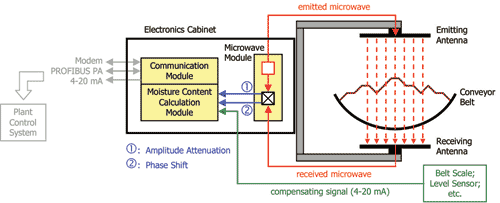
Figure 1
An online moisture analyzer is a device that permits direct measurement of moisture content for specific applications by using methods others than LoD. Many industrial processes may call for the use of on-line moisture content measurement, for example: measuring coffee freshness (food process), determining the composition of paint (chemical process), and determining the water content in ores (mineral process). The relevance of use of a moisture analyzer depends on the nature and objectives of the process. Some key applications of such analyzers in mineral processes are:
- Equalization of bulk ore masses in dry basis for mass balance and production accounting.
- Operating control of dilution water in SAG and ball mills.
- Operating control of filtration, dewatering, drying and pelletizing processes.
- Monitoring the moisture content of ores regarding an upper limit, in ship loading operations.
This paper outlines the application of an on-line moisture analyzer in a bauxite ore processing plant.
Models for Microwave Moisture Measurement
Microwaves are electromagnetic waves with frequencies in the range 0.3–300 GHz. When a microwave passes through any material, its energy is partially dissipated (absorbed) by the material, causing a decrease in wave intensity (attenuation) and an offset in wave displacement (phase shift). The degree by which the wave is attenuated and phase-shifted by a specific material depends on the wave frequency and on the electrical properties of the material, such as its “dielectric constant.” The higher the dielectric constant of a material, the higher the energy dissipation (attenuation and phase shift) of microwave passing through it. Water has a higher dielectric constant than many common materials, and is highly interactive with microwaves. The basic model equation for microwave-based moisture measurement can been seen in Model 1.
Model 1

Where:
mc: moisture content by weight (%w)
M: wet mass of material (Kg)
α: microwave amplitude attenuation (dB)
φ: microwave phase-shift (rad)
α0, bi: model parameters
The model does not consider ore density explicitly. Although different densities change microwave amplitude and phase in different ways, this effect is embodied by the mass M. The calibration of the model above is developed as follows: ore samples are dried, weighed, and then artificially moistened by the addition of known masses of pure water, yielding a set of sample wet masses {Mi} with moisture contents {mci}. This is best done in laboratory, under controlled conditions. The samples are subjected to a microwave analyzer, and the resulting set of microwave attenuations {αi} and phase-shifts {φi} are measured. After these laboratory tests, the set of experimental data values {mci, Mi, αi, φi} is statistically analyzed to detect and eliminate possible outliers. The remaining valid data set is then used in a multivariate regression to determine values of the parameters α0, b1, and b2 that best fit the experimental data.
To improve measurement accuracy, some moisture analyzers have been designed to operate with two simultaneous microwave signals of different frequencies, leading to a more complex model, as seen in Model 2.
Model 2
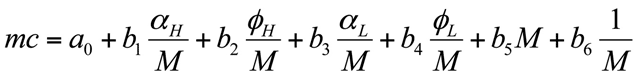
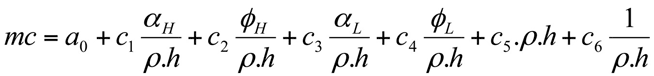
Model 2 is used in applications in which the material mass M can be directly measured and provided for the model. If this is not the case, but the material density ρ is almost constant (has a small variance), Model 2 can be rewritten in terms of material level (bed depth) h, as seen in Model 3.
Model 3
Where:
mc: moisture content by weight (%w)
M: wet mass of material (Kg)
ρ: material density (g/cm3)
h: material level (mm)
αH: higher frequency microwave amplitude attenuation (dB)
φH: higher frequency microwave phase shift (rad)
αL: lower frequency microwave amplitude attenuation (dB)
φL: lower frequency microwave phase shift (rad)
α0, bi, ci: model parameters
The calibration of Models 2 and 3 follows the same guidelines as for the simpler Model 1, with the difference that a larger set of sample data values is needed for the multivariate regression calculations, due to the greater number of parameter values to be determined.
Microwave Moisture Analyzers for Mineral Applications
An important attribute of microwaves is that they are highly interactive with water. The measuring principle of moisture content of a material relies on sensing the attenuation and the phase-shift of a microwave signal passing through the material. A microwave moisture analyzer, shown in Figure 1, is an instrument that implements this principle. The analyzer has two microwave antennas—one for transmitting and one for receiving—which are placed around the material flow (normally in a conveyor belt) in a upper-lower orientation.
The transmitting antenna generates a known reference microwave signal which passes through the material, is attenuated and phase-shifted, and then reaches the receiving antenna. By comparing the received signal with the emitted signal, the analyzer determines the overall attenuation and phase-shift of the microwaves due to their interactions with both the material and its water content. To distinguish the attenuation and phase-shift due to only the water content in the material, the analyzer needs information about the amount of material, which is provided by a “compensating signal” from an independent instrument. All the signal processing and model calculations are performed by a specialized algorithm implemented in the analyzer electronics, which also yields the moisture measurements to the plant control system.
Some advantages of microwave moisture analyzers are:
- Representative non-contact measure ment: Microwaves perform a reliable non contact measurement because they are not subject to wear by contact. And, because they pass through the bulk of the material being measured, a very representative measurement can be obtained.
- Accurate measurement: Microwave moisture analyzers can reach accuracies from 0.5% to 0.1%w, for 1-standard-deviation confidence, when they are well designed and calibrated. This accuracy is very suit able for process control and production accounting in mineral applications.
- Wide measurement range: Microwave moisture analyzers can work within measurement ranges as wide as 0% to 90%w. Such a range can meet a large variety of applications.
- Suitable for harsh environments: Harsh industrial conditions are a major challenge for instrument reliability, mainly in mineral applications. Microwave moisture analyzers are usually robust and can handle severe applications, with proper installation design.
One limitation of microwave moisture analyzers is:
- Hard-to-perform calibration: A well designed, installed, configured and calibrated microwave moisture analyzer sys tem can be reliable for long periods.
However, due to its relative complexity and the inherent need for material sam pling, handling, and drying, calibration of such analyzers is a multi-step, hard-to perform and time-consuming task. This limitation becomes a problem when, for whatever reason, the analyzer requires frequent recalibrations. The best way to avoid this problem is through care in the design, installation, calibration and maintenance of the equipment.
The HYDRO Bauxite Plant
HYDRO’s bauxite processing plant, located 60 km from Paragominas in Pará state, Brazil, is shown in Figure 2. Plant construction ran from August 2004 to December 2006, and commissioning began in March 2007. The plant receives raw bauxite ore from an open-pit mine, and performs a set of comminution and separation processes to produce bauxite slurry, which is pumped through a 243-km-long pipeline from the plant site to the HYDRO Alunorte alumina refinery, in the city of Barcarena, Pará.

Figure 2
Measuring the moisture content of the ore at the input of grinding circuits allows for accounting of the actual dry mass fed to the circuits, from which the mass balance and the mass recovery of the circuits can be computed. The mass recovery, given by the ratio between the input dry ore fed to the grinding circuits and their output slurry mass produced, is a key performance indicator of the plant, since it indicates how much of the total input ore has been converted into product slurry.
The moisture analyzer was originally installed on belt conveyor TC-121-02 (See Figure 2) in order to take advantage of an existing belt scale on this conveyor, to provide the compensating signal required by the analyzer. However, after the analyzer had been installed, its moisture measurements were found unreliable when compared with laboratory sample values. Further investigation of the entire system indicated incorrect belt scale measurements were caused by mechanical misalignment in the conveyor structure and belt sliding, hence compromising the moisture measurements. To overcome those problems, two steps were taken: to relocate the analyzer to another conveyor, TC-123-02 (See Figure 2), still at the input of a grinding circuit; and to use another compensating method for the analyzer, to avoid it being “slave” of unreliable belt scales. The new method chosen was material level compensation.
Calibration and Installation of the Moisture Analyzer
The first step in the design of a moisture analyzer system is the selection of the model that best suits the intended application. All further work involving the building and calibration of the system will depend on the chosen model. It is also necessary to define the moisture range in which the analyzer is intended to work because the set of sample moisture values to be used in the model building must cover appropriately the intended moisture range of the application. In this project, this was done by checking historical moisture data from the plant laboratory database, for the conveyor on which the moisture analyzer would be installed. It was found that the nominal moisture range of the ore was 10.5–13.5%w, with eventual higher values of no more than 17.5%w. Hence, the intended calibration range of the analyzer was chosen as 0–18%w.
The analyzer was originally delivered to work with Model 2. However, the compensating method would be changed from material load compensation to material level compensation, and hence Model 3 had to be developed. Development of a new model is done in three steps.
Step 1: Pre-Calibration (Initial Model Building)—The pre-calibration is the initial determination of values for the parameters ({a0, ci} in Model 3). This is best done with the moisture analyzer at a laboratory workbench. Using a set of material samples with known moisture contents mci, achieved by the addition of known masses of pure water to the dry masses of the ore samples, each sample was put inside a non-metallic (fiberglass) box to form a layer of ore with known height (level) hi. The box was then placed between the microwave antennas of the analyzer to sense the microwave attenuation αi and phase-shift φi corresponding to the moisture content mci, level hi, and density ρ of the ore sample. For this step, it’s not necessary to take the ore samples from stop belt sampling. One can use ore collected from other easily accessible locations, like the plant stockyard, provided that the collected material has similar properties (particle size distribution and density) to the material carried by the conveyor on which the analyzer would be installed.
This initial model building is difficult due to the need for so many ore sample creations, for better representativeness within the intended measuring range for the analyzer (0–18%w). This task used seven reference moisture values (0, 7, 9, 11, 13, 15, and 17%w), five reference levels (within 60–390 mm), two sample box positions (front and rear), and five sample measurement collection, resulting a total of 350 sample measurements of microwave attenuation and phase-shift values. It took seven days, with 12 hours/day of work, to complete the tasks. Figure 3 shows some pre-calibration data for the chosen set of reference moisture values. The graphs show the relationship between the quantities αL/M and φL/M versus the moisture content mc, for model (2).
 |
 |
| Figure 3 A | Figure 3 B |
After sample data collection in laboratory, the set of experimental data values {mci, ρ, hi, αi, φi} was statistically analyzed to detect and eliminate possible outliers. The remaining data set was then used in a multivariate regression to determine values of the model parameters {α0, ci} that best fit the experimental data. The model was then loaded into the analyzer electronics by the manufacturer, through Ethernet communication, from a laptop running a proprietary configuration software.
Step 2: On-Site Calibration (Model Refinement)—Having concluded the pre-calibration step, the moisture analyzer was installed on conveyor TC-123-02. An overview of the installation is shown in Figure 4.
Because of some differences between actual field conditions and the laboratory conditions of the pre-calibration step, an on-site calibration for model refinement is necessary. This refinement is simply an adjustment on the model parameter values {α0, ci} determined in the pre-calibration step.
While the analyzer is running, a set of composite samples is taken from conveyor belt stops, and their corresponding moisture values measured by the analyzer are recorded. The samples are sent to laboratory to be analyzed through the LoD method. A measurement check is performed based on the deviations between the analyzer measurements and the laboratory results. If necessary, the model parameter values {α0, ci} are adjusted to better match the laboratory results.
The greater the number of samples collected from the conveyor, the more consistent the calibration would be. Ideally, a minimum of 30 samples should be collected. In this work, however, due to restrictions to stop the conveyor belt, a set of only 14 composite samples of wet ore, each one involving three cuts, were collected. The sampling uncertainty (σsampling) is given by the root mean squared error (RMSE) of all the cut sample values of all the composite samples, and resulted as σsampling = 0.391%w.
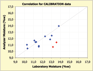
The criterion to consider a cut sample value as an outlier was a cut sample deviation greater than two standard deviations. One of the samples was regarded as an outlier and removed from the sample data set. The remaining 13 valid sample results are shown in Figure 5(a).
 |
 |
| Figure 5 A | Figure 5 B |
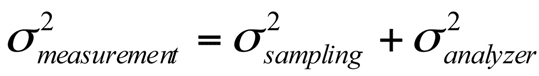
For each of those valid composite samples, the error εi was computed between the moisture value from the analyzer and its corresponding result from laboratory analysis. The sample errors had an average value με = –0.449%w and a standard deviation σε = 0.995%w. Two of the valid samples (indicated by red points in Figure 5(a)) were out of the 2-standard-deviation region (|εi | > 2σε) and were regarded outliers. Excluding those outliers, the remaining 11 sample values are the valid set of values from which the measurement uncertainty should be determined. The measurement uncertainty or accuracy (σmeasurement) is given by the root mean squared error (RMSE) between the valid composite sample values from the analyzer and their corresponding values from laboratory. It resulted as σmeasurement = 0.577%w. Finally, the measurement uncertainty is a quadrature combination of the sampling uncertainty and the calibration uncertainty or analyzer accuracy (σanalyzer) as seen in Equations 5 and 5a.
Equation 5
Equation 5 A

Equation 5 B
![]()
The moisture measurement accuracy required by the plant operations was ±0.5%w. Since the accuracy achieved by the analyzer had met this requirement, the calibration was regarded as suitable.
Step 3: On-site Verification (Model Validation)—After on-site calibration is achieved, the model should be validated. This is done with a new set of material samples, collected in the same way as for the on-site calibration step. If the sample measurements from the analyzer are consistent with their corresponding sample moisture results from laboratory, then the model is considered valid. Otherwise, a new model calibration should be done.
A set of 10 three-cut composite samples of wet ore were collected from conveyor belt stops, and the moisture measurements from the analyzer associated to those samples were recorded. The sampling uncertainty for all of the cut sample values of all the composite samples resulted as σsampling = 0.717%w. This uncertainty was greater than the one from the on-site calibration, suggesting differences in the sampling, storage or laboratory practices between the two sampling campaigns. None of the composite samples presented cut sample deviations greater than two standard deviations (no cut sample outliers). All the 10 valid sample results are shown in Figure 5(b).
The sample errors εi between each moisture value from the analyzer and its corresponding result from laboratory analysis had an average value με = –0.354%w and a standard deviation σε = 1.258%w. One of the valid samples (indicated by the red point in Figure 5(b)) was out of the 2-standard-deviation region (|εi| > 2σε) and was regarded an outlier. Excluding this outlier, the remaining 9 sample values were used to determine the measurement uncertainty, which resulted as σmeasurement = 0.855%w. Hence, the analyzer accuracy can be seen in model 5b.
Since this verified analyzer accuracy resulted close to the accuracy from the calibration step, and still within the ±0.5%w requirement from the plant operations, the analyzer was regarded as well calibrated.

Figure 6
Operating Results
The analyzer yields its moisture measurements to the plant process control system (PCS) through an analog 4–20 mA signal. Figure 6 shows a trend graph of the moisture content of the bauxite ore over a period of 20 minutes. Such variations are virtually impossible to detect from stop-belt sampling of ore, but are easily detected by an on-line analyzer.
Trend graphs, like in Figure 6, are useful to understand short-term variations of the moisture content of the ore. To understand long-term variations, a histogram is best. Figure 7 shows a histogram of moisture for a period of 475 hours (≈ 20 days). The probability of the moisture being lower than 10.5%w was 1.11%; whereas the probability of being in the range 10.5–13.5%w was 95.81%; and the probability of being greater than 13.5%w was 3.08%.
The histogram above clearly indicates that the moisture distribution is not Gaussian. Its asymmetrical form was expected because, from the plant process conditions, it is virtually impossible for the ore to have moisture values lower than 9%w, but there are many conditions that can increase the natural moisture content of the ore, such as rain or wash water on the conveyors. The statistics of this distribution are: median λ = 11.18%w, mean μ = 11.37%w, and standard deviation σ = 0.83%w. Before the implantation of the moisture analyzer, the nominal moisture value officially considered by the plant operations was 12%w. However, the median and mean values computed from the analyzer measurements should be more confident.

Figure 7
Care is Crucial
Microwave moisture analyzer systems can be used advantageously provided that they are designed and calibrated thoroughly. The key issues for a successful calibration of a microwave analyzer are the collection of representative sets of samples, and careful laboratory analysis, to provide consistent sample data for the calibration.
To obtain useful results, it’s vital that the facility staff properly maintain the equipment. There are many reasons why workers may be reluctant to take proper care of analyzer systems; classic excuses include: “It’s difficult to stop the conveyor to take material samples,” and “It’s difficult to take too many material samples,” or “We would waste too much time to recalibrate the analyzer” and “The analyzer is more complex than other instruments.” Those issues must be addressed to keep an analyzer operating effectively.
Although this application pertains to bauxite ore, most of the information presented here can be applied to different ores or bulk materials.
Sidney A.A. Viana is a process control project specialist at Norsk HYDRO ASA’s Paragominas, Brazil, bauxite operations. He can be contacted at sidney.viana@vale.com.