


Understanding material flow from the mine through Vale’s Paragominas processing plant and pipeline to the customer’s delivery station
By Sidney A.A. Viana
Bauxite ore is the basic raw material for the aluminum production chain, which has four major steps, normally implemented as separate industrial plants: processing of the raw ore from bauxite mines to produce concentrated ore with specific quality requirements; refining of the concentrated bauxite ore through the Bayer process to produce high-purity smelter-grade alumina; electrolytic reduction of the smelter-grade alumina in high-current electrolytic furnaces to produce primary aluminum in the form of ingots, billets or slabs; and smelting and conformation of the primary aluminum to create end-user aluminium products.
The first step is performed by ore processing plants by means of several types of mineral processing facilities, such as crushing, milling, screening, hydrocycloning and thickening, among others. Normally, the main process variable in a mineral plant is the mass of ore processed in each facility. Correct understanding of the mass processed through an entire plant is fundamental for performance accounting of the process.
Actual measured process data usually contain measurement errors due to less-than-ideal or defective aspects of the measurement systems, or of the process itself. Examples of these aspects are mechanical vibrations corrupting the mass measurement by a belt scale; turbulence in a stream, affecting its flow measurement by a magnetic flowmeter; poorly calibrated field instruments; electromagnetic interferences; or bad signal transmission.
Measurement errors are classified into two groups: random errors and gross errors. Random errors are those caused by random and generally unpredictable and uncontrolled aspects of the process, so they can be regarded as statistical variations of the measurement values. Gross errors are those caused by systematic and usually defective characteristics of the process or equipment, and they can be regarded as biased deviations in the measurement values. Although it’s virtually impossible to fully eliminate measurement errors, they can be reduced by means of improvements in the measurement systems or in the design of the process.
Measurement errors will prevent the measured data from satisfying the process constraints that describe the process, such as its mass or energy conservation laws. These errors can deteriorate the performance of the process, leading it to non-economical or even unsafe conditions. Therefore, it’s important to continuously assess the quality of the measured data, in order to detect and compensate for measurement errors, since they cannot be fully eliminated from the process.
The methodology for quality assessment of measurement data comprises two major steps: Gross Error Correction and Data Reconciliation. The correction of gross errors involves three steps: detection, identification and elimination of gross errors.
Data Reconciliation and Mass Balance
The concept of data reconciliation is to adjust measured process data and to estimate unmeasured ones (where possible), so that they fully satisfy the process constraints described by a process model. In other words, since the measured data don’t usually satisfy the process constraints, due to the presence of measurement errors, the data reconciliation will use those measured data as an initial guess and then refine their values so that the process constraints become fully satisfied. The resulting values are called “reconciled values.”
Mathematically, data reconciliation is an optimization problem by which an optimal set of “better” data values (the reconciled values) should be computed from a given set of original data values, according to the process model and constraints, assuming that only random errors are present in the original data. The optimization criterion is the minimization of the overall error between the reconciled and the original data, subjected to the process constraints.
A critical aspect of data reconciliation is the assumption that only random errors, and not gross errors, should be present in the data. If this assumption is not true, the reconciliation might lead to large adjustments in the data, and the resulting reconciled values may be inaccurate or even infeasible. Therefore, the detection, identification and elimination of gross errors are prerequisites for data reconciliation.
Data reconciliation problems are referred to according to the nature of the process that they deal with. For example, “mass balance,” for reconciliation of mass data; “energy balance,” for energy data; “heat balance,” etc.
In practice, data reconciliation has been widely used in chemical, petrochemical, food and beverage processes, where the need for consistent and accurate data is critical for quality control, performance accounting and legal compliance. In mineral processes, unfortunately, data reconciliation is not yet consistently used, although its importance is known.
The general relationship of a balance problem is given by equation 1:
Input − Output − Storage + Generation − Consumption = 0
Where:
Input: the total quantity that enters the system.
Generation: the total quantity produced inside the system.
Consumption: the total quantity consumed inside the system.
Storage: the total quantity accumulated inside the system.
Output: the total quantity that leaves the system.
(“Quantity” may be an amount of mass, energy, heat, etc.)
In equation 1, the generation and consumption terms are normally associated with chemical reactions, where the consumption can be the mass of a reactant, and the generation can be the mass of a product from the reaction. On the other hand, in a purely physical process with no chemical reactions, like most of the mineral processes, those terms are not present.
The Paragominas Plant
The former Vale’s bauxite processing plant, located 60 km from Paragominas, Brazil, was commissioned in March 2007. The plant receives raw bauxite ore from an open-pit mine, and performs a set of comminution and separation processes to produce bauxite slurry that is pumped through a 243-km-long pipeline, from the plant site to the customer site (Alunorte), in Barcarena.
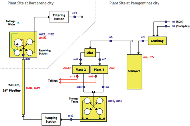
Figure 1—Overall diagram of the bauxite production chain, with regards to its main mass variables.
Figure 1 shows an overall diagram of the entire production chain, from the mine and processing plant, to the pipeline and customer delivery station, with regards to the main mass variables.
The mass m1 is the mass of raw ore dumped by trucks into the primary crushers. The mine operations typically perform about 800 dumping events per day, making it impractical to weigh all the trucks feeding ore to the crushers. Because of this, m1 was fixed on an average basis: the average mass per truck was determined by weighing a small set of trucks (e.g., 20 trucks) and then used as a fixed value. Thus, the mass of the Run of Mine (RoM) ore fed to the crushers in a certain period is estimated by multiplying the number of dumping events in the period and the fixed average mass per truck. The same was done for the mass m2. All of those calculations were performed automatically by the mine’s dispatch system.
The average mass per truck is affected by three main factors: the density of the ore (geological aspect); the filling of the truck bucket (human aspect); and the rainfall (environmental aspect), which affects the moisture of the ore. As a consequence, the average mass per truck can vary significantly over different periods, with a standard deviation of about 15%, which was taken as the typical uncertainty for m1 and m2.
The masses m3 (production from primary crushing), m6 (reclaimed from the stockyard), m7 (feed for plant line 1), and m11 (feed for plant line 2) are all masses of bulk ore transported by belt conveyors, and are directly measured on wet basis by existing belt scales. On the other hand, the masses m9, m13, m17 and m20 are dry basis masses of slurry calculated from their volume (V), density (ρ), and solids concentration (cs) measurements, according to equation 2:
m = V ρ cs
where the volume V and the density ρ are measured, respectively, by magnetic flowmeters and nuclear density transmitters; and the solids concentration cs is determined straightforward from ρ as given by equation 3:
cs = ρ (ρs – ρl )
ρs (ρ– ρl )
where ρs is the density of the solids in the slurry, assumed fixed as ρs = 2.6 metric tons per cubic meter (mt/m3); and ρl is the density of the liquid (water) in the slurry, assumed fixed as ρl = 1 mt/m3.
Equations (2) and (3) are normally implemented in the plant’s control system, which receives the volume and density measurements from the respective field instruments, and then computes the respective mass. When there’s no density transmitter, as for m9 and m13, the density is determined from slurry samples collected manually from the streamline at regular intervals, but at the expense of a much slower measurement rate than if a field instrument have been available.
In the terminology of mass balance, any part of a system that defines a mass conservation relationship (equation 1) is called a node. According to Figure 1, the entire bauxite processing chain has eight nodes, with the following nodal equations to be satisfied:
• Node 1 (primary crushing): the mass of crushed ore (m3) must be equal to the total mass of raw ore fed to the crushing (m1 + m2), assuming that the crushing does not accumulate mass:
m1 + m2 = m3
• Node 2 (the stockyard): the final mass stock (m5) must be equal to the initial stock of mass (m4) plus the difference between the input mass (m3) to, and the output mass (m6) from the Stockyard:
m5 = m4 + m3 – m6
• Node 3 (the silos): the total mass fed to the plant lines 1 and 2 (m7 + m11) must be equal to the input mass to the silos (m6):
m7 + m11 = m6
• Nodes 4 and 5 (plant line 1 and plant line 2): for each plant line, the input mass (m7 or m11) must be equal to the sum of its respective production mass (m9 or m13), reject mass (m10 or m14), and variation of accumulated mass (Δm8 or Δm12):
m7 = m9 + m10 + Δm8;
m11 = m13 + m14 + Δm12
• Node 6 (the storage and pumping station): the final stock of product mass (m16) must be equal to the initial stock (m15) plus the difference between the total input mass (m9 + m13) and the pumped output mass (m17) from the pipeline:
m16 = m15 + m9 + m13– m17
• Node 7 (the pipeline): the final contained mass (m19) in the pipeline must be equal to the initial contained mass (m18) plus the difference between the pumped input mass (m17) and the delivered output mass (m20):
m19 = m18 + m17 – m20
• Node 8 (the receiving station): the delivered mass (m20) must be equal to the variation of stored mass in the tanks (m22 – m21) plus the variation of accumulated mass (Δm23) and the filtered product mass (m24):
m20 = m22 – m21 + Δm23 + m24
Let’s denote the number of measurements by Nm, and the number of nodal equations by Nc. From the above discussion, we have: Nm = 24 measurements and Nc = 8 nodes. The set of nodal equations can be expressed in matrix form where C is the nodal matrix, M is the vector of measurements, and K is the vector of nodal errors. In the ideal case where the measurements satisfy exactly all the nodal equations, K is a null vector. But in practical situations, where the measurements contain measurement errors, K is not identically null. The data reconciliation intends to solve the following problem: for a given C and a measured M, how to adjust M so that K becomes identically null?
Mass Recovery
A basic key performance indicator (KPI) of a mineral processing unit is its mass recovery, which is the ratio between the production mass and the feeding mass to the unit. For example, suppose that a mineral processing facility is fed with F tons of ore, generates P tons of product, and R tons of reject material, with no internal accumulation of mass. Then, its mass recovery is: MR = P/F×100%. A high mass recovery means that most of the feeding mass is converted into product, whereas a low mass recovery means that most of the feeding was lost as reject and not converted into product. In other words, the mass recovery is a measure of the production efficiency of the process.
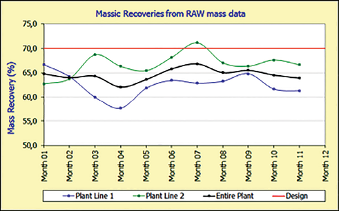
The Paragominas processing plant project was intended to achieve a mass recovery of about 70%, but due to several problems in its design, implantation and maintenance after four years of operations, its actual mass recovery calculated from the original mass measurements resulted around 65%. This value indicates that 35% of the input mass to the plant is lost as reject (tailings), when the suitable value from the project should be around 30%. But when calculating the mass recovery from reconciled mass values, the recovery was closer to 60%. Considering an annual production of 7,556,000 mt at a product value of $36.59/mt, the undesirable loss of 10% in mass recovery correspond to a loss of $27.65 million per year in revenues. This is a clear example on how the use of data reconciliation to estimate optimized values of mass will allow a more accurate knowledge of the mass recovery, which is a key indicator of the plant performance.
Solving the Mass Balance Problem
The presence of gross errors in some mass measurements of the bauxite processing chain have been observed since the early stages of data processing. Inspections on the field instruments of the plant indicated several problems affecting them, such as calibration issues, incorrect installation, poor preventive maintenance, etc. Several meetings with maintenance personnel were held to discuss those problems and define action plans to solve them. Unfortunately, no effective solution was achieved in the subsequent three years after startup. Due to such poor maintenance practices and the time constraints with fixing a lot of instruments, the correction of gross errors was ignored, and the data reconciliation was performed using the original measurements from the instruments. This is not the right approach, but it was the best available at the time.
Data Reconciliation
The data reconciliation problem was solved using the method of Lagrange Multipliers [2,4,7], summarized bellow.
Let’s denote the vector of measurements as M, whose elements are the measurements of each mass variable. And let’s denote the corresponding vector of percent uncertainties as UP. Then, the vector of absolute uncertainties UA is given by equation 4:
UA = UP⊗M
where the operator “⊗” means an element-wise multiplication.
The reconciliation matrix is given by equation 5:
H(Nm + Nc) x (Nm + Nc) = [ DCT
C0 ]
where: D is a Nm×Nm diagonal matrix whose k-th diagonal element is given by: dkk = 2/(UA(k))2. C is the Nc×Nm nodal matrix. 0 is a Nc×Nc null matrix.
The solution is given by equation 6:
S = H-1 x M
where the first Nm elements of the vector S are the reconciled measurements given by equation 7:
R(k) = S (k) ǀ 1 ˂ k ˂ Nm
and the remaining elements in S are the Lagrange multipliers given by equation 8:
L(k) = S(k) ǀ Nm + 1 ˂ k ˂ Nm + Nc
The vector of reconciliation adjustments, which are the corrections made on the original values, are given by equation 9:
A = R – M
The computational implementation of the data reconciliation strategy described above was done in VBA (Visual Basic for Applications) for use in Microsoft Excel.
Results
To evaluate the performance of the entire bauxite production chain, the data reconciliation was performed on a monthly basis for a period of 11 months of plant operation. The results of the data reconciliation for the sixth month are shown in Table 1. The two columns at right of the table show the elements of the vector of nodal errors K, for the original and reconciled mass values. Notice that all elements of K become null for the reconciled values, as expected.
To better understand the meaning of the reconciliation adjustments, they were classified into four levels, as described in Table 2. Figure 3 shows the adjustments from Table 1 in a bar graph, according to the levels in Table 2. Different levels of corrections were made by the data reconciliation on the original measurements. The higher is the adjustment, the less reliable the original measured value was.
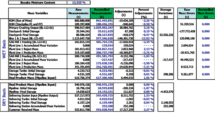
Table 1—Mass balance results for the sixth month.

Table 2—Adjustment levels.
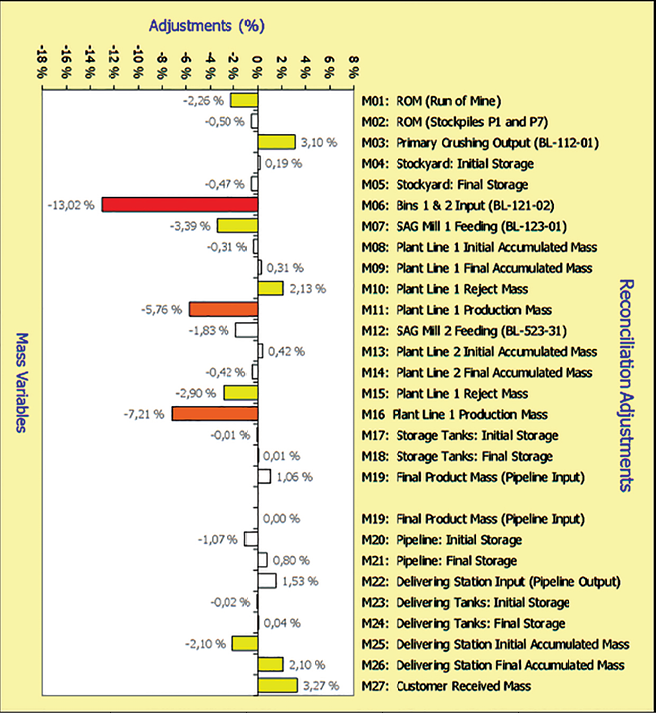
Figure 3—Adjustments in the mass values from the data reconciliation for the sixth month.
Usefulness of the Data Reconciliation Results for Process Management
Most of the benefits of the data reconciliation relies on the improved accuracy of the reconciled results, allowing better knowledge of the behavior of the process and the performance of the plant. Some of these benefits are:
1. Detection of failures in measuring devices: a high reconciliation adjustment is normally a consequence of gross errors caused by a defective measurement. Therefore, the adjustments resulted from the data reconciliation indicate the quality of their respective measuring devices. This information can be useful to guide maintenance actions and to establish a quality control of the measurements. As an example, Figure 3 shows an excessive adjustment (the red bar) for the belt scale BL-121-02. Its original measurement was adjusted in -13.02% by the data reconciliation. It was verified through a field inspection that the encoder (speed sensor)of the belt scale was damaged, thus causing a gross error on the original measurement.
2. Better accounting of the production: the reconciled values of the mass of product delivered to the customer are more suitable for custody trans- fer purposes, due to their improved accuracy.
3. Estimation of unmeasured variables: the ability to estimate unmeasured vari- ables, including leakage flows of ma- terial in the process is another major advantage of the data reconciliation. With enough measurement redundan- cy, data reconciliation can provide reasonable estimates for the amounts of materials that are not directly mea- sured. In this work, examples of un- measured variables are m10 and m14; and examples of leaks or losses are Δm8, Δm12, and Δm23.
4. Improved accuracy for calculations of mass recovery: since the mass re- covery is the ratio between the produc- tion mass and the feeding mass, its accuracy depends on the quality of these two mass values. The original measurements, which contain mea- surement errors, often lead to wrong values of mass recovery. Therefore, the use of the reconciled mass values improves the confidence of the mass recovery results.
As an example, Table 3 shows the mass recovery results from the original and the reconciled mass values, for the seventh month. For plant line 2, the mass recovery of 71.17% calculated from the original masses seems impractical, since the plant was designed to achieve a maximum recovery of 70%. Moreover, although the entire plant output (m9+ m13) and the pipeline input (m17) must have the same value, their mass recovery resulted different because of the presence of measurement errors. But the exact same mass recovery value resulted when calculated from the reconciled masses, as expected. This is an example on how the original measurements, that are inherently corrupted by measurement errors, can lead to wrong values of something else that would be calculated from them.
Figure 4 shows the mass recovery values along the 11 months evaluated, for the original and reconciled values.
This work presented the use of data reconciliation to perform the mass balance of a mineral processing chain. The results obtained show that most of the benefits of data reconciliation rely on the improved accuracy of the reconciled results, allowing better knowledge of process behavior. This is important because one cannot control or manage well what is not measured well.
The optimized accounting for material entering, being stored, and leaving a process, helps to identify where losses or mis-measurements may be occurring within the process plant, which might be unknown, or difficult to measure. The conservation laws used in the accounting depends on the context of the problem, but all revolve around mass conservation, i.e., that matter cannot disappear or be created within the process.
The correction of gross errors requires continuous and focused efforts from maintenance and engineering departments. Unfortunately, in mineral processing plants, those efforts are often neglected, thus preventing the process and operations teams to work with the best possible measurement data. This is not a technical problem, but a management problem. Each plant or industrial unit must define a suitable management strategy to deal with this problem.
Sidney A.A. Viana is a specialist automation engineer at Vale’s Ferrous Automation Engineering Department. He can be reached at sidney.viana@vale.com.
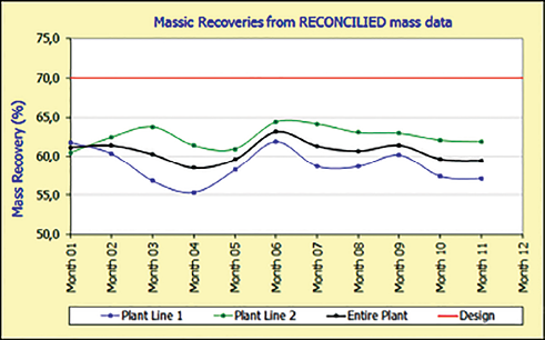
Figure 4—Mass recovery results. (a-left) From the original mass values. (b-right) From the reconciled mass values.

Table 3—Mass recovery results computed from original and reconciled data values, July 2010.
Acknowledgement
The author would like to thank Henrique C. Santos (mine engineer), Clóvis W. Maurity (geologist), Dario de Castro (geologist), Obadias Farias (pipeline operation analyst), and Fábio S. Nogueira (pipeline operation technician), for their input during the development of this work.
References
1. Caulkins, J.P.; Morrison, E.L. & Weidemann, T. “Spreadsheet Errors and Decision Making: Evidence from Field Interviews.” Heinz Research. Carneggie Mellon University. 2005. http://repository.cmu. edu/heinzworks/24.
2. Kreiszig, E. “Advanced Engineering Mathematics,” seventh edition. John Wiley & Sons, 1993.
3. Mah, R.S.H.; Stanley, G.M. and Down- ing, D.W. “Reconciliation and Recti- fication of Process Flow and Inven- tory Data.” Ind. & Eng. Chem. Proc. Des. Dev., vol.15, 175-183, 1976.
4. Narasimhan, S. & Jordache, C. “Data
Reconciliation and Gross Error De- tection: An Intelligent Use of Pro- cess Data.” Gulf Publishing Co., 1999.
5. Reilly, P.M. and Carpani, R.E., “Appli- cation of Statistical Theory of Adjust- ment to Material Balances.” 13th
Canadian Chemical Engineering Con- ference, Ottawa, Canada, 1963.
6. Sorensen, H.W. “Least Squares Estimation: From Gauss to Kalman.” IEEE Spectrum Magazine, vol.7, n.7, pp.63–68, 1970.
7. Wills, B.A. & Napier-Munn, T.J. Wills’ “Mineral Processing Technology.” (Chapter 3: Metallurgical Accounting, Control and Simulation), seventh edi- tion. Butterworth-Heinemann, 2006.